Magnetic Field Exposure Assessment in Electric Vehicles

Andrea Vassilev, Alain Ferber, Christof Wehrmann, Olivier Pinaud, Meinhard Schilling, and Alastair R. Ruddle, Member, IEEE

Abstract—This article describes a study of magnetic field expo- sure in electric vehicles (EVs). The magnetic field inside eight dif- ferent EVs (including battery, hybrid, plug-in hybrid, and fuel cell types) with different motor technologies (brushed direct current, permanent magnet synchronous, and induction) were measured at frequencies up to 10 MHz. Three vehicles with conventional powertrains were also investigated for comparison. The measure- ment protocol and the results of the measurement campaign are described, and various magnetic field sources are identified. As the measurements show a complex broadband frequency spectrum, an exposure calculation was performed using the ICNIRP “weighted peak” approach. Results for the measured EVs showed that the exposure reached 20% of the ICNIRP 2010 reference levels for general public exposure near to the battery and in the vicinity of the feet during vehicle start-up, but was less than 2% at head height for the front passenger position. Maximum exposures of the order of 10% of the ICNIRP 2010 reference levels were obtained for the cars with conventional powertrains.

Index Terms—Electric vehicle, human exposure, hybrid vehicle, magnetic field.

 

 

Introduction

PUBLIC expectations to move toward the electrification of road transport are driven by a multitude of factors and con- cerns, which include climate change, primary energy depen- dence, and public health. On the other hand, there is widespread public concern regarding the possible adverse effects of elec- tromagnetic fields (EMF), particularly low-frequency magnetic fields. The occupants of vehicles with electric powertrains will be exposed to low-frequency magnetic fields arising from cur- rents flowing in the high-voltage power network, traction bat- teries, and associated devices such as inverters and electrical machines. Thus, there is a need to properly assess the level of magnetic field exposure that may result in electric vehicles

 

Manuscript received September 2, 2013; revised April 14, 2014; accepted August 29, 2014. This work was supported in part by the European Commu- nity’s Framework Programme (FP7/2007-2013) under grant agreement number 265772.

Vassilev is with the CEA LETI, Grenoble 38054, France (e-mail: andrea. vassilev@cea.fr).
Ferber is with the SINTEF, Oslo 0314, Norway (e-mail: alain.ferber@ sintef.no).
Wehrmann and M. Schilling are with the Technische Universita¨t Braunschweig, Braunschweig 38106, Germany (e-mail: c.wehrmann@tu-bs.de; m.schilling@tu-bs.de).
Pinaud is with the G2ELAB, Grenoble 38402, France (e-mail: olivier. Pinaud@g2elab.grenoble-inp.fr).
R. Ruddle is with the MIRA Limited, Nuneaton CV10 0TU, U.K. (e-mail: alastair.ruddle@mira.co.uk).

Color versions of one or more of the figures in this paper are available online at http://ieeexplore.ieee.org.

Digital Object Identifier 10.1109/TEMC.2014.2359687

(EVs), which include battery powered, hybrid, and fuel cell variants.

The International Commission on Non-ionizing Radiation Protection (ICNIRP) has recommended limits for exposure to static [1] and time-varying [2] EMFs. These limits aim to pro- vide protection from well-established acute physiological ef- fects of EMF exposure, which include electro-stimulation of nerves (relevant for frequencies from 1 Hz to 10 MHz) and heat- ing of body tissues (for frequencies from 100 kHz to 300 GHz). The recommendations relating to electro-stimulation effects, which are the primary interest in this study, were revised by ICNIRP in 2010 [3].

The exposure limits are actually specified in terms of in-body quantities that are not easy to determine. Consequently, ICNIRP has derived more readily measureable field reference levels from the exposure limits. It is considered that if the exposure envi- ronment complies with the field reference levels then it can be assumed that the exposure limits will not be breached. Exceed- ing the field reference levels does not necessarily mean that the exposure limits are also breached, but it is deemed that more de- tailed investigation is required in order to establish compliance with the exposure limits.

In situations of simultaneous exposure to fields of differ- ent frequencies, these exposures are considered to be additive in their effects [2], [3]. Thus, the more frequencies that are present, the lower the levels that can be tolerated for any of them relative to the field reference levels. Furthermore, the in- fluence of other fields that may be present in the environment also impact on what can be tolerated from equipment generating fields that people may be exposed to. This is very different to the evaluation of electromagnetic emissions against equipment EMC requirements, where compliance with the limits at each frequency is considered independently of all other frequencies, and independently of the other equipment that may be present in the intended operating environment.

The field reference levels vary with respect to frequency and are valid only for pure sinusoidal signals. In the case of nonsinu- soidal exposures, ICNIRP has proposed two exposure criteria that should remain below 100% to avoid undesirable electro- stimulation effects. The first one (which also applies in the case of separate sinusoidal sources at multiple frequencies) consists in adding the ratios of the different spectral component (SC) magnitudes of the field in the environment to the field refer- ence levels. A similar approach is also described in the IEEE standards relating to human exposure [4], [5], although in these documents the frequency range for the evaluation of electro- stimulation threats is up to 5 MHz.

 

 

0018-9375 © 2014 IEEE. Personal use is permitted, but republication/redistribution requires IEEE permission.

See http://www.ieee.org/publications standards/publications/rights/index.html for more information.

The main drawback of this criterion for nonsinusoidal signals is that it assumes that all frequency components add in phase. This assumption is acceptable for signals with a limited number of SC, but for broadband signals this procedure could lead to an unnecessarily conservative exposure assessment. In [6] it is shown that for a measured field spectrum with SC that are all less than 1% of the ICNIRP 1998 [2] reference levels for the general public, the first criterion would suggest that the exposure is 634%. Relative to the ICNIRP 2010 reference levels the SC are all less than 0.1% of the general public recommendations, but the first criterion would suggest that the exposure reaches 99% of the general public recommendations.

For these reasons a second criterion is defined by ICNIRP (the “weighted peak” approach [3]) in which a time-varying exposure measure is derived from an inverse Fourier transform that take into account the phase of each SC. This approach is more general and can be applied for every kind of magnetic field waveform. Using this approach, [6] indicates that the maximum value of the time-varying exposure measure is less than 20% of the ICNIRP 1998 reference levels for the general public, and less than 5% of the ICNIRP 2010 field reference levels.

Published data concerning field exposure in EVs is somewhat scarce, and not always appropriate for assessment against the ICNIRP field reference levels. For example, the research con- ducted in [7] characterized the magnetic fields associated with various form of transportation. The results showed that EVs have a magnetic field spectrum roughly similar to conventional ve- hicles (CVs), but no exposure assessment was calculated. This study also found no evidence for measureable electric fields associated with vehicles in the band 5 Hz to 3 kHz.

In a more recent paper [8], it is reported that magnetic fields measured in a hybrid car are much lower than the ICNIRP 1998 field reference levels, but no results taking into account addi- tive effects were presented. Maximum fields of ~15 μT (in the band 0.01–5 kHz) were recorded in a hybrid bus at the seat lo-

cated closest to power cables during acceleration, deceleration, and driving at 25 km/h [9], but no information regarding the time variation of the magnetic field is provided.

Two hybrid cars were measured in [10], which indicates that the exposure could reach 80% of the ICNIRP 1998 reference levels for the general public in the vicinity of the passenger’s feet during braking and acceleration. In [11] the second criterion was employed to evaluate measurements at 12 points that represent various body parts from head to foot for front and rear occupant location in five cars with motor powers ranging from 15 to 147 kW. Time-domain measurements were carried out over 1 s periods under constant drive conditions for frequencies from 1 Hz to 100 kHz. Exposure relative to the ICNIRP 1998 general public reference levels was reported to reach a maximum value of around 15% in the vicinity of the front occupants’ feet. These authors also report maximum exposure measures approaching 20% of ICNIRP 1998 general public levels at head height in a hybrid bus [12].

This paper describes the measurement of eight different EVs and three CVs, with characteristics as outlined in Table I, as well as the calculation of realistic exposure measures from these measurements using the second criterion (i.e., the ICNIRP

 

TABLE I

Summary of Measured Vehicles

 

Car code	Powertrain type	Electric motor technology	Power (kW)	Energy (kWh)
EV#1	Battery	Brushed dc	11	10
EV#2	Plug-in hybrid	Permanent magnet	30	5
EV#3	Small hybrid	Induction	10	0.7
EV#4	Battery	Permanent magnet	10	14
EV#5	Battery	3-phase asynchronous	34	24.5
EV#6	Battery	Permanent magnet	40	24
EV#7	Fuel cell	Permanent magnet	100	1.4
EV#8	Battery	Permanent magnet	35	16
CV#1	Gasoline	–	75	–
CV#2	Gasoline	–	66	–
CV#3	Diesel	–	125	–

 

 

 

 

weighted peak approach). Section II outlines the measurement protocol and Section III summarizes the main sources of mag- netic field in vehicles. The exposure calculations are presented in Section IV, and Section V summarizes the conclusions.

 

 

1. Measurement Protocol
2. Measurement Setup
   • Sensors: Four kinds of sensors were used:
     • Low-frequency (LF) 3-axis magnetic field sensors (Flux- gate magnetometers):

±    ±      ±

• Bartington MAG-03 (bandwidth 0–3 kHz; range: 100, 250 or 500 μT; noise < 10 pT/√Hz);

1. Sensys FGM 3-D/100 (0–1.2 kHz).

• High-frequency (HF) 3-axis magnetic field sensors:
  1. Narda EHP-50D (5 Hz to 100 kHz);
  2. Spectran NF-5035 (1 Hz to 10 MHz).
• Current sensor Fluke i310s (range 0–300 A, 0–20 kHz) used to establish the correlation between the magnetic field and the current flowing in the high-voltage power

±

• Acceleration sensor (STMicroelectronics, model LIS3LV02DL, range 6 g), used to establish the relationship between acceleration and power flow.

• Acquisition system: The LF sensors and the current sen- sor were connected to an OROS analyzer (model name OR36) whose main functions were to:
  • low-pass filter the signals (cut-off frequency 2 kHz);
  • sample the signals (sampling frequency 12 kHz);
  • provide concurrent recording of the

The HF sensors had their own sampling and recording system.

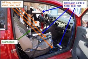
• Mannequin and Sensor Positions: In order to mount the different magnetic sensors and to ensure reproducible position- ing, a nonmagnetic mannequin was developed (see Fig. 1), in- spired by [7] and [13]. As tests were made while driving the cars, the mannequin was installed on the front passenger seat. The mannequin was equipped with three LF and three HF sensors located near the head, seat, and foot A fourth LF mag- netic field sensor was placed above the main battery in the trunk. The current sensor was placed on one of the battery cables.

 

 

1. Laboratory Tests

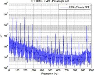
For some of the EVs, laboratory tests were carried out in order to characterize the magnetic field emissions of all of the on-board electrical equipment. The car was raised on a lift in order to be able to place sensors below the car; everything was switched off except for the item under test. The magnetic field was then measured and this process repeated for every other item of equipment. This procedure is quite time consuming but very informative. For example, it revealed that a very specific harmonic spectrum is due to the steering pump of EV#1. This is illustrated in Fig. 2, which shows the root sum square (RSS) of the Fourier transforms obtained from the waveforms recorded for each of the three orthogonal components of the magnetic field.

 

1. Outside Tests

Outside tests are the most important because they are the most representative of real-world driving conditions. The main prob-

 

 

 

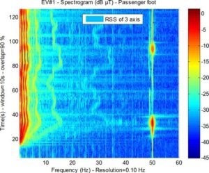
Fig. 3. Spectrogram showing evidence of two 50 Hz high-voltage power lines.

 

 

lem with these tests is that there are several external magnetic perturbations that could influence the results. The approaches used for identifying these perturbations, and then performing the tests, are described later.

• Identifying external magnetic perturbations: There are several sources of external magnetic perturbation in the en- vironment, such as stationary or moving ferromagnetic masses (e.g., manhole covers, railway lines, other cars), as well as 50 Hz power distribution equipment (high-voltage transmission lines, power transformers etc.).

These initial tests were carried out within a specific area with restricted access (for example the CEA complex in Grenoble) because the number of other cars was then limited. A specific driving route was defined in this controlled area and the car repeated the journey several times under different driving con- ditions (low and high speed, acceleration and deceleration). If the results contained a magnetic field feature that occurred ev- ery time at the same place, it was concluded that this field was due to an external perturbation. For example, a spectrogram ob- tained from a sensor located on the floor of EV#1 is illustrated in Fig. 3, which shows a clear permanent 50 Hz signal with two strong features located at around 30 and 100 s (on the vertical time axis). These features are probably due to two high-voltage 50 Hz power lines passing under the driving route.

Once the external magnetic perturbations were identified, fur- ther tests were performed on a normal road.

• On Road Tests: On road tests were performed which in- volved driving with maximum acceleration and deceleration in order to ensure maximum positive (traction) and negative (re- generative brake) currents. A straight road is better because in this case the magnetic fields due to the earth and due to the in- duced magnetization of the car are constant during the For the first few cars, measurements were also carried out on a steep slope and at high speed on a highway. However, it appeared that these two driving conditions did not generate higher fields

 

 

than for acceleration and deceleration on the flat road. For the remaining cars, therefore, the on road tests were performed only on a flat road and at moderate speeds (0–60 km/h).

III. IDENTIFICATION OF MAIN SOURCES OF MAGNETIC FIELD
In this section, the main sources of magnetic field are listed, grouped by frequency content and presented in order of increas- ing frequency.

A. Traction Currents
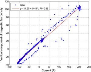
It is well known that a current flowing through a wire or a loop generates magnetic field. Our measurements show that, for most of the cars, the high-voltage power network acts as a current loop. Moreover, the magnetic field close to the battery could be important: the ratio between the induced magnetic field and the traction current was found to be in the range 0.2– 1 μT/A, depending on the car. Therefore, if the traction current has variations up to 300 A, the magnetic field could also have variations of up to 300 μT. An example is shown in Fig. 4, where the vertical component of the magnetic field at each point in time is plotted versus the corresponding current. In this case, the traction current varies from 100 A to + 200 A whereas the magnetic flux density is in the range 40 μT to +100 μT; hence the field–current ratio is of the order of 0.5 μT/A.
The magnetic field due to traction currents also presents a high spatial variability. In EV#1, for example, the magnetic field in the vicinity of the passenger’s foot ranges from 30 to 130 μT within distances of a few tens of cm. This is due to the fact that when two cables carrying opposite currents are close together (as is the case in the central tunnel of EV#1), the resulting magnetic field is minimized. But when the cables diverge (as is the case in the engine bay of EV#1), the field can increase significantly.
Although this field is important, it is far below the ICNIRP general public limit of 40 mT for static fields [1] and below the

 

 

 

 

 

 

 

 

 

ICNIRP general public limits for frequencies below 1 Hz [2]. Nonetheless, traction current transients with SC above 1 Hz may contribute significantly to the in-vehicle magnetic field exposure [6].

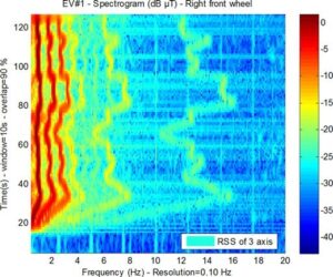
B. Wheels
The permanent magnetization of steel belted tires is a well- known source of in-vehicle magnetic fields (see [14], [15]). Our measurements show that this phenomenon is responsible for a magnetic field inside the car of up to 2 μT at the wheel frequency fw (which ranges from 0 to 20 Hz for speeds ranging from 0 to 130 km/h). There are also several harmonics present at lower intensities. The spectrogram shown in Fig. 5 (in dBμT) was obtained from a sensor placed near the passenger’s foot location in EV#1, close to the front right-hand wheel. The electric motor
was switched off and the car was manually pushed at low speed (~4–5 km/h) corresponding to fw ~1 Hz. This clearly shows a fundamental signal ~1μT at fw as well as the higher harmonics f2 , f3 , f4 , f8 , and f16 with decreasing magnitudes. As the
ground was not flat, it was difficult to maintain a constant speed, which is why the fundamental frequency fluctuates over time.

C. Internal Combustion Engine
Measurements on the hybrid car EV#2 show that there is a correlation between the rotational frequency fm (varying up to 100 Hz) of the internal combustion and the magnetic field signals. This could be due to the motion of the pistons. The
magnitude of the associated magnetic signal was ~150 nT at frequency 2fm in this case.

D. Specific Equipment
Specific equipment of the car may also generate magnetic fields. The magnetic field emissions from the power steering pump (500 W, 12 V) of EV#1 have already been reported

(see Fig. 2). This equipment can generate fields up to 1 μT inside the car at frequencies in the range 0.5–1 kHz (see Fig. 6). For EV#2, just after an accelerator pedal release, a wide-band magnetic signal of ~1μT at frequencies up to 400 Hz was ob- served on the sensor above the battery. It is believed that this

signal may be due to the regenerative brake. On EV#3, an un- explained coupling between an equipment working at constant frequencies (50 and 100 Hz) and the motor (whose fundamental frequency f₁ is proportional to the wheel frequency, such that f₁ = 4f_w ) was found to lead to fields of the order of 0.5 μT at frequencies up to 600 Hz.

 

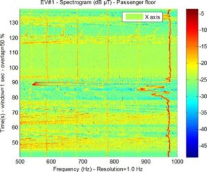
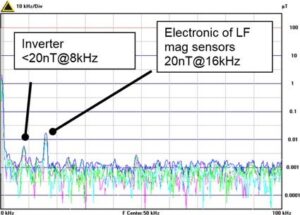
1. Inverter

A power inverter is an electrical device that converts direct current (dc) to alternating current (ac). In EV, it is typically characterized by a switching frequency of around 10 kHz. To deal with these frequencies, it is necessary to use the HF sensors. These measurements were carried out for only four of the cars (EV#1–EV#4). Below 200 kHz, the field level was less than 20 nT; the maximum values observed in this frequency range (see Fig. 7) were at

• 7–9 kHz, probably due to the inverter;
• 16 kHz, due to the LF sensor

Between 200 kHz and 10 MHz, the field level is a little higher but still low (less than 60 nT). A harmonic spectrum can be observed, but it is difficult to establish its origin.

 

1. Summary

The contributions from the different sources above 1 Hz that were identified are summarized in Table II and in Fig. 8. In this figure, each source is represented by a horizontal solid (blue or black) colored line. The vertical position indicates the maximum field measured, while the length indicates the frequency range. The dotted red line connects the different sources and forms a spectral envelope of the measurements. It can be seen that

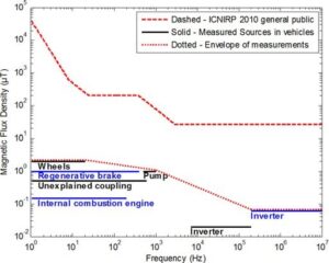
this envelope is decreasing with increasing frequency. Most of the magnetic field sources (wheels, brake, and steering pump) produce frequencies ranging between a few Hz and 1 kHz, with magnitudes of 0.1–2 μT. At frequencies above a few kHz, the magnetic field is less than 100 nT and only the inverter was identified as a source from the vehicles.

Compared to the ICNIRP 2010 reference levels defined for the general public and for pure sinusoidal signals [3], which

is plotted in Fig. 8 using dashed red line, the envelope of the magnetic field emissions is roughly two decades lower than the

 

where WF_j represent the peak amplitude of weighting func- tion at frequency f_j and the terms ϕ_j represent the corre- sponding phase values. The parameters ϕ_j are specified as zero when B_R (f_j ) is constant, π/2 when B_R (f_j ) 1/f , π when B_R (f_j ) 1/f ² , and π/2 when B_R (f_j )  f (see Appendix A of [3]).

∝         −               ∝

∝

ICNIRP recommends that the summation goes from 1 Hz (corresponding to j = p) to 10 MHz (corresponding to j = n). In this paper it was found that the magnetic field levels decreased rapidly for frequencies above 1 kHz. Therefore, the exposure sum ranges from 1 Hz to 2 kHz, and only the signals from the LF sensors are used. The weighted signal is then simply compared to the reference level at frequency f_r .

we,f r

R

r

1

2

B          (t) < √2B (f ),       for t ∈ [t ; t ] .              (4)

 

of magnitude of the exposure is 1% of the reference levels. As already noted in Section I), it is necessary to take into account the additive effects of all frequencies from all sources in order to assess the exposure (see Section IV).

Dividing by the right term of the inequality, we obtain a time-varying exposure function c(t), independent of f_r that is required to be <1 in order to guarantee compliance with the basic restrictions:

 

 

1. Exposure Calculations
2. Weighted Peak Approach for Nonsinusoidal Exposures

The weighted peak exposure criterion defined by ICNIRP in

f_j =2 kHz

¯ Σ

c(t) =

¯ f_j =1 Hz

B_j BR,j

. cos(2πtf_j + θ_j + ϕ_j )¯ ≤ 1,

 

¯

for t ∈ [t₁ ; t₂ ] .      (5)

 

the case of nonsinusoidal exposures (see [3] and [16]) is appli- cable for arbitrary magnetic field waveforms B(t). The general idea is:

• defining a reference frequency f_r ;
• computing from B(t) a weighted signal B_{we,f r} (t) that takes into account the frequency dependence of the mag- netic field reference level B_R (f );
• comparing this weighting signal to the reference level

B_R (f_r ) at reference frequency.

If it is assumed that B(t) is periodic on the measured interval [t₁ ; t₂ ], then B(t) may be approximated by the n spectral com- ponents (SC) derived from B(t) by means of a discrete Fourier transform. Thus,

Σ √

n

 

B(t) =               2B_j . cos (2πtf_j + θ_j )                       (1)

j =1

 

where j is the summation index of the SC (including the dc component), B_j represent the RMS amplitudes of the SC at frequency f_j , and θ_j correspond to the phases of the SC.

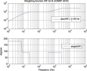
The weighting function WF is defined (see Fig. 9) such that the gain is inversely proportional to the chosen magnetic field reference levels B_R (f ) and the corresponding phase values are

related to the frequency dependence of BR (f ):
WF (f, fr ) = BR (fr )/BR (f ). (2)

The weighted magnetic field waveform can then be calculated
as
n
Bwe,f r (t) = WFj  2Bj . cos (2πtfj + θj + ϕj ) (3)
j =p
Electro-stimulation effects are instantaneous, with the result that ICNIRP recommend that the basic restrictions (and by im- plication, the field reference levels) should not be time averaged. For convenience, therefore, the time-varying exposure measure can be summarized in terms of its maximum instantaneous value EC (for exposure criterion):

EC = max {c(t)} ,       for t ∈ [t₁ ; t₂ ] .                      (6)

 

1. Practical Implementation

The ICNIRP recommendations give very few details con- cerning the practical implementation of this calculation. For example, it is not clear how to:

• choose t₁ and t₂ ;
• compute the SC in case of a nonperiodic signal;
• deal with the three components of a magnetic field;
• select a sampling rate for digitizing the

For the first point, the criterion has been calculated with dif- ferent bounds t₁ and t₂ in order to verify that the criterion does not change.

For the second point, the fact that the signal may not be peri- odic can lead to spectrum leakage, i.e., signal energy smearing out in the frequency domain. Another consequence is that the

TABLE III
SUMMARY OF EXPOSURE RESULTS

Car code Maximum exposure Position
EV#1 14.3% Front passenger foot
EV#2 17.8% Above rear battery
EV#3 7.9% Above rear battery
EV#4 5.9% Rear passenger foot
EV#5 4% Front passenger seat
EV#6 3.2% Front passenger seat
EV#7 2.1% Front passenger seat
EV#8 2.7% Front passenger foot
CV#1 2.7% Front passenger seat
CV#2 9% Left rear passenger seat
CV#3 10% Left rear passenger seat

 

temporal function c(t) is perturbed near its bounds (at t1 and t2 ). One way to deal with this problem is to use short-time Fourier transform (STFT) instead of a simple FFT. This solution has been successfully tested, but it is quite time consuming. A sim- pler solution is to discard a small region around each bound (e.g., q = 2% of signal length l) when calculating the exposure measure:
EC = max {c(t)} , for t ∈ [t1 + ql; t2 − ql] . (7) For the third point, it is assumed that for each of the M
sampled field component the weighted field waveforms and their associated time-varying exposure measures ci(tk ) are computed according to (3) and (5), respectively. For each time sample tk , the root sum square (RSS) value then is calculated from the three orthogonal components in order to obtain the multidimensional exposure C(tk ), where

 

M
C(tk ) =
i=1

(ci (tk ))2 . (8)

Finally, the worst case instantaneous exposure for the entire magnetic field is obtained by applying (7) to C(tk ) to obtain the maximum value.

C. Results
For each car, simple drive cycles were investigated includ- ing acceleration and deceleration phases. The exposure was computed as outlined earlier from measurements at the four positions: head, seat, foot, and above the battery. The maxi- mum exposure levels and locations results are summarized in Table III.
The main results for the EV examples are as follows.
1) The highest values, between 14% and 18% of the ICNIRP 2010 general public reference levels, appear on EV#1 and EV#2, when the engine is switched on.
2) For every EV, the highest values were reached near the battery and the foot of the driver or passenger.
3) The maximum exposure at head-height for the front pas- senger was found to be 1.5% of the ICNIRP 2010 general public reference levels.

For the CV examples, the highest values were around 10% of the ICNIRP 2010 general public reference levels, and were also linked with vehicle start-up and braking events.

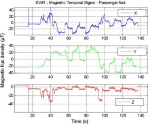
As an example, Fig. 10 shows the whole magnetic field wave- form for a short journey with EV#1, as recorded by a sensor located in in the vicinity of the passenger’s foot. It can be seen that there is a sharp peak in the magnetic field waveforms on the X and Z axes when the vehicle is switched on (around time 15 s).

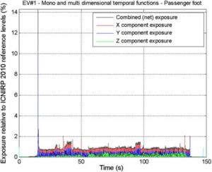
The exposure measures c_i(t_k ) obtained from the three orthog- onal field component waveforms are shown in Fig. 11, along with the corresponding RSS value C(t_k ). A sharp peak can also be seen at the same time (at around 15 s) and the peak exposure reaches almost 15%. Finally, Fig. 12 shows the detail around the peak of the X component of the field and the corresponding

 

 

 

 

 

 

 

 

 

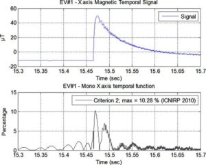
exposure measure cX (tk ). It can be seen that the rapidly ris- ing edge in the X component of the magnetic field waveform is a major contributor (at ~10%) to the overall exposure (see Fig. 11).

V. CONCLUSION
The magnetic field of eight different EVs (including battery powered, hybrid, and fuel cell variants) with different types of motor technology (brushed dc, permanent magnet synchronous, and induction) were measured in the frequency range from dc to 10 MHz. Three vehicles with conventional powertrains were also investigated for comparison purposes. A suitable measure- ment protocol was developed, based on the use of a mannequin to ensure reproducible positioning of the field sensors.
The main magnetic sources of the EV were identified: at very low frequency (<1 Hz), magnetic fields of several hundreds of μT can be encountered mainly due to traction currents and induced magnetization effects. Most of the magnetic sources (wheels, regenerative brake, steering pump, and combustion en- gine) are found at frequencies between a few Hz and 1 kHz, with magnitudes between 0.1 and 2 μT. Above 1 kHz, the magnetic field is less than 100 nT and only the inverter was identified as a source from the vehicle.
As the measurements showed a complex broadband fre- quency spectrum, an exposure calculation was performed ac- cording to the ICNIRP 2010 recommendations [3]. It was found that the highest exposure for the EVs that were tested was less than 20% of the field reference levels for general public expo- sure, and corresponded to vehicle start-up. For all of the cars in the EV sample, the highest values were found near the battery and in the vicinity of the feet of the driver or front passenger. The maximum exposure at head height for the front passenger head was found to be less than 2% of the ICNIRP 2010 field reference levels for general public exposure.

For the cars with conventional powertrains, maximum expo- sures of the order 10% were obtained, depending on the position of the sensor.

ACKNOWLEDGMENT
The authors are grateful for the support and contribu- tions of other members of the EM-Safety project consor- tium, from Centro Ricerche Fiat (Italy), Leibniz University of Hanover (Germany), IPM (Italy), MIRA (UK), Prysmian (Italy), TAMAG Iberica (Spain), and the University of Torino (Italy). Further information can be found on the project website (www.sintef.no/Projectweb/EM-Safety).

REFERENCES
[1] ICNIRP, “Guidelines on limits for exposure to static magnetic fields,”
Health Phys., vol. 96, no. 4, pp. 504–514, Apr. 2009.
[2] ICNIRP, “Guidelines for limiting exposure to time-varying electric, mag- netic, and electromagnetic fields (up to 300 GHz),” Health Phys., vol. 74, no. 4, pp. 494–522, Apr. 1998.
[3] ICNIRP, “Guidelines for limiting exposure to time-varying electric and magnetic fields (1 Hz to 100 kHz),” Health Phys., vol. 99, no. 6,
pp. 818–836, Dec. 2010.
[4] IEEE standard for safety levels with respect to human exposure to elec- tromagnetic fields, 0–3 kHz, IEEE Standard C95.6-2002, Oct. 23, 2002.
[5] IEEE standard for safety levels with respect to human exposure to electro- magnetic fields, 3 kHz to 300 GHz, IEEE Standard C95.1-2005 Apr. 19, 2005.
[6] A. R. Ruddle, L. Low, and A. Vassilev, “Evaluating low frequency mag- netic field exposure from traction current transients in electric vehicles,” in Proc. 12th Int. Eur. Symp. Electromagn. Compat., Brugge, Belgium, Sep. 2013, pp. 78–83.
[7] F. M. Dietrich and W. L. Jacobs, “Survey and assessment of electric and magnetic field public exposure in the transportation environment,” US Department of Transportation, Federal Railroad Administration, Rep. PB99-130908, Mar. 1999.
[8] M. N. Halgamuge, C. D. Abeyrathne, and P. Mendis, “Measurement and analysis of electromagnetic fields from trams, trains and hybrid cars,” Radiation Protection Dosimetry, vol. 141, no. 3, pp. 255–268, 2010.
[9] M. Pous, A. Atienza, and F. Silva, “EMI radiated characterization of an hybrid bus,” in Proc. 10th Int. Eur. Electromagn. Compat. Symp., York, U.K., Sep. 2011, pp. 208–213.
[10] E. Karabetsos, E. Kalampaliki, G. Tsanidis, D. Koutounidis, N. Skam- nakis, T. Kyritsi, A. Yalofas, “EMF measurements in hybrid technology cars”, presented at 6th Int. Workshop Biol. Effects Electromagn. Fields, Bodrum, Turkey, Oct. 2010.
[11] G. Schmid, R. U¨ berbacher, and P. Go¨th, “ELF and LF magnetic field exposure in hybrid- and electric cars,” in Proc. Bioelectromagnetics Conf., Davos, Switzerland, Jun. 2009, pp. 9–3.
[12] R. U¨ berbacher, G. Schmid, and P. Go¨th, “ELF magnetic field exposure
during an inner-city hybrid bus ride,” in Proc. Bioelectromagnetics Conf., Davos, Switzerland, Jun. 2009, pp. P–23.
[13] A. Brecher, D. R. Disk, D. Fugate, W. Jacobs, A. Joshi, A. Kupferman, R. Mauri, and P. Valihura, “Electromagnetic field characteristics of the tran- srapid TR08 maglev system,” US Department of Transportation, Federal Railroad Administration, Rep. DOT-VNTSC-FRA-02-11, May 2002.
[14] S. Milham, J. B. Hatfield, and R. Tell, “Magnetic fields from steel-belted radial tires: Implications for epidemiologic studies,” Bioelectromagnetics, vol. 20, no. 7, pp. 440–445, 1999.
[15] S. Stankowski, A. Kessi, O. Be´cheiraz, K. Meier-Engel, M. Meie, “Low frequency magnetic fields induced by car tire magnetization,” Health Phys., vol. 90, no. 2, pp. 148–153, Feb. 2006.
[16] K. Jokela, “Restricting exposure to pulsed and broadband magnetic fields,”
Health Phys., vol. 79, no. 4, pp. 373–388, 2000.

Andrea Vassilev received the mechanical engineering degree, in 1996, from Ecole Centrale de Lyon, France.
From 1996 to 2001, he was with PSA Peugeot Citroen, as a Mechanical Sim- ulation Engineer. Since 2001, he has been with CEA-LETI, Grenoble, France, a research institute for electronics and information technologies.

Alain Ferber received the M. Sc. degree in Cybernetics from The Norwegian Institute of Technology, in 1976.
He is currently a Senior Scientist in the Department of Optical Measurement Systems and Data Analysis at SINTEF, Oslo, Norway.

 

 

Christof Wehrmann received the M.Sc. degree in electrical engineering, from the Technische Universita¨t (TU) Braunschweig, Braunschweig, Germany, in 2011. He is currently working toward the Ph.D. degree at Institut fu¨r Elektrische Messtechnik und Grundlagen der Elektrotechnik at the TU Braunschweig.
Since 2011, he has been with the Institut fu¨r Elektrische Messtechnik und Grundlagen der Elektrotechnik at the TU Braunschweig as a Research Assistant.

 

 

Olivier Pinaud received the electrical engineering degree from the Grenoble Institute of Technology, Grenoble, France, in 2010. Since 2011, he has been working toward the Ph.D. degree on electromagnetic computation at Grenoble Electrical Engineering Laboratory (G2ELAB), France.

Meinhard Schilling received the diploma in physics, in 1989, and the Ph.D. degree (Dr. rer. nat), in 1992, both from the Universita¨t Hamburg, Hamburg, Germany.
In 1998 after habilitation he was with the University Hamburg as Privat- dozent. Since 2001, he has been a Full Professor and Head of the Institut fu¨r Elektrische Messtechnik und Grundlagen der Elektrotechnik, at the Technische Universita¨t Braunschweig.

 

 

Alastair R. Ruddle (M’10) received the B.Sc. degree in physics from the Uni- versity of Bristol, Bristol, U.K. and the Ph.D. degree in electronic and electrical engineering from the University of Loughborough, Loughborough, U.K.
Since 1996 he has been a computational electromagnetics specialist with MIRA Limited, Nuneaton, U.K., an automotive research and technology orga- nization. Prior to this he carried out research in the defense and power industries.